views
- Start by selecting blank cells that mirror the same amount as your original cell set.
- Enter "
=TRANSPOSE(" to apply the function to all selected cells. - Press Ctrl+⇧ Shift+↵ Enter to run the function.
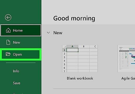
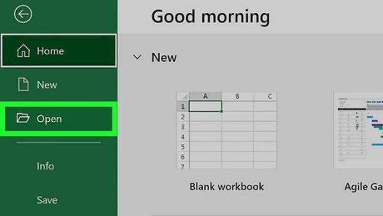
Open your document in Excel. You can find this program in your Start Menu or Applications Folder. You can either open your document from Excel by clicking Open from the File tab, or you can right-click the file in your file browser and click Open With.
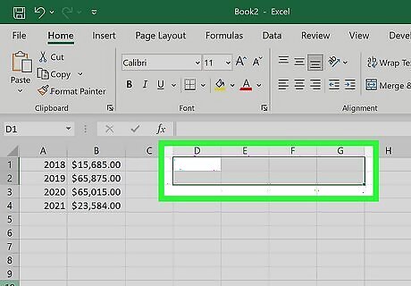
Select blank cells that mirror the same amount of your original cell set. For example, if you have 4 cells of data presented vertically that you want to display horizontally and 4 cells of data you have horizontal that you want vertical, make sure you select the same amount of blank cells (8) so they can be transposed.
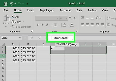
Enter "=TRANSPOSE(". Type this while you have the cells selected and it will apply to all the cells.
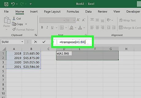
Type the range of cells you want to transpose. For example, if the 8 cells of data are in A1-B4, you'll enter "=TRANSPOSE(A1:B4)". Don't press Enter/Return yet.
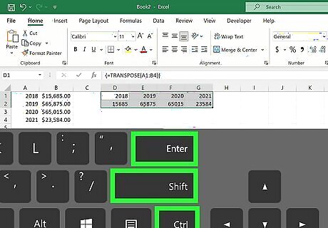
Press Ctrl+⇧ Shift+↵ Enter. Since you're using an array formula (which is a formula that gets applied to more than one cell), you'll need to press Ctrl + Shift + Enter instead of just Enter. If you don't like those results, you can try using the copy and paste/transpose method.


Comments
0 comment