views

Open a new XL workbook: From the desktop, on the dock, click on the green Excel "X"; Go to menu item File and hold it down with mouse; Move the mouse down to where it says "New Workbook" or "Open a New Workbook" and release the mouse button or pressure to select the menu option; or Alternatively, go to the Applications folder in your hard drive icon by double-clicking that and double-clicking on the Applications folder; Find Microsoft Office, and select it; Find Excel within it, and double-click on it; Proceed to Open a new workbook from the File menu. You may encounter an interim window with spreadsheet icons on it. Select New Workbook.
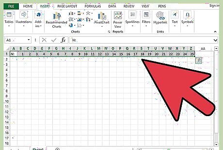
Enter into the new workbook the Column and Row Headers for the Times Table: Select Preferences, under Excel, and in General, uncheck Use R1C1 reference style; in Calculation, check Automatically; Enter to cell A1, w/o quotes, "n: " (with the trailing space) and do menu Format Cells Alignment right; Enter to cell B1 the value 1; Select with the mouse by constantly holding it down as you move over the columns in row 1, cell range B1:Z1; Do menu Edit Fill Series (in Rows, Linear) (Step value = 1), OK. You will have the values from 1 to 25; Do menu Insert Name Define name n to the cell range B1:Z1, without quotes. Select cell range A1:Z1. Do menu Format Cells Fill canary yellow and then Font dark blue to the selection range. Select the cell range of rows in column A (by dragging the mouse on it) from A2:A25; Enter, w/o the external quotes, the formula, "="a="&B2" and do menu item Edit Fill Down; Select cell range B2:B25 and enter 2 to cell B2, then do menu Edit Fill Series (in columns, linear, with Step value 1), OK. The result will be in column B you have the values 1 to 25, and in column A the Row Headers a=2, a=3, a=4 ... down to a=25. Select or stay on the cell range B2:B25 and do menu Insert Name Define name a to the cell range selected, just the letter a, without quotes. Do menu Format Cells Fill canary yellow, Font red for the selection B2:B25.
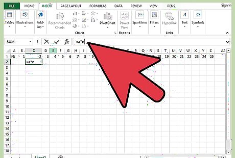
Enter the Multiplication Table with a simple copied formula of your Defined Name variables, n and a. Enter to cell C2, w/o quotes, the live formula "=a*n"; Do menu Edit Copy cell C2 and select the entire table cell range C2:Z25 by dragging mouse over it diagonally down and to the right holding down the Shift Key; Do menu Edit Paste. The result should be a filled in Times Table with 625 (=25*25) in the bottom right-hand corner.
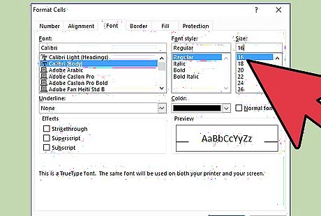
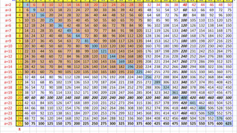
Format the Multiplication Table Select in the far upper worksheet corner above the 1 of Row 1 and to the left of A of column A to select the entire worksheet simultaneously; Do menu Format Cells Font size 16 or 18 -- make it large enough so you will enjoy reading it. Select the cells that you will memorize, say up to your 12x12's or 15x15's -- so select cell range C2:P15 for your 15's and do menu Format Cells Fill, light brown. If you are only asked to memorize through your 12's, select cell range C2:M12 and do menu Format Cells Fill light brown. By the way, you can easily expand the definitions of a and n and create a larger chart to access and learn from. Or, you can change the Step Value increment to 5 or 25 or 100, etc. It is very easy to remember your 20s and to count by 20s. If you like the idea of adding that as a memory aid, select cell range C20:Z20 and Format Cells Font bold AND italic. Do the same for cell range U2:U25; Select cell range C2:Z2 and do menu Format Cells Font red and bold (this relates to the Chart we're going to make shortly); Select cell range C25:Z25 and do menu Format Cells Font bold (this also has to do with the Chart); Select, holding down the Command key, the squares of the numbers in a diagonal from top left to bottom right, not letting go of the Command key, from 4 to 9 to 16 to 25 ... all the way down diagonally to 625. When those are all selected, you cannot copy such a selection but you can still format it. Do menu Format Cells Fill light blue and Font bold. Those are the numbers squared.
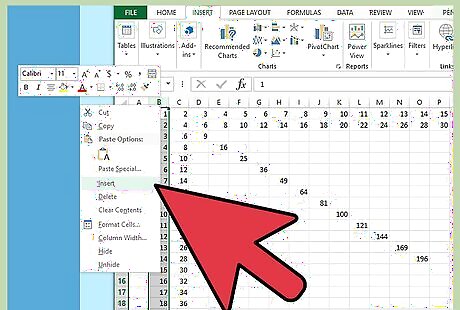
Extra Credit (if you choose to do so) -- Create the Chart and Learn about Slope: Select Row 2 by selecting the Row# which is 2 at the left of the spreadsheet. Do menu Insert Rows. One row should be inserted. Select cell range A2:Z26 and then use the Ribbon or menu Chart and create a new Chart and select, All, Scattered, Smoothed Line Scattered for the chart type -- a new chart should appear atop your worksheet, so move it off to the right by grabbing with the mouse inside the chart border and dragging rightwards and up or down until it's located in a good spot. Select Row 2 again and do Edit Delete; Your new Chart should read the chart series reference down the right, for example, a=2, then below it a=3 ... all the way down to a=25. Double-click on the bottommost line (or plot series) of the chart and in the dialog box that appears set Line color to Red; Double-click on the topmost line (or plot series) of the chart and in the dialog box that appears set Line color to Black; notice that over in the series references, they are "upside-down" and that the top one for a=2 refers to the bottom red series line, and that the bottom one refers to the top series line for a=25. Reason that this is because 2 has less "slope" than the steeper "slope" for 25. Calculate actual slope with the formula (y2 - y1)/(x2 - x1). You have just created an {x, y} Cartesian Graph. Select cell AA1 and type Y, which pertains to all those columnar values. Format Cells Font Bold. Select cell B26 and type X, which pertains to those vertical values. Now the rightmost Y is actually point Y25 and the bottom X is point X25. You will learn to adjust the slope formula to the endpoints when you first study slope of lines, so we're going to change the formula to (Y25 - Y1)/(X25 - X1). Filling in the values of those data point references, we have Y25=50, Y1=2, X25 = 25 and X1=2. The formula thus becomes (50-2)/(25-2) or 48/23 = 2.087, which is slope m1, the slope of the red series line. For the black series line, Y25=625, Y1=25, X25=25 and X1=2, so the formula's values become (625-25)/(25-2), or 620/23 which equals 26.957 or slope m25. You can perform this division right in Excel by preceding it with an equals sign, somewhere off to the side. A slope m of 1 is a straight 45 diagonal from {X1, Y1} = {0, 0} through each pair of similar matching numbers, like {4, 4} or {25, 25). Then the formula become (25-0)/(25-0) = 1/1 and slope m=1. You can see that the product of a and n for the first 25 numbers produces a range of slopes from 2.087 up to 26.957, which is fairly steep. Your chart probably does not show how truly steep it is because it is not a square of 625 x 625 but is cut off so that it's only got a width of 30. If we were to change the horizontal axis by double-clicking on it and setting the Max to 625, you'd see how very steep a slope of nearly 27 actually is, and the lines would be all crowded together. That is why the lines "fan out" as they do, because their slopes m are different and the chart is foreshortened. In school, you may learn one formula for a line is y= mx + b or you may learn it as y= ax +b; m and a stand for the slope in either case. The slope is determined by (Y2 - Y1)/(X2 - 1 ), not by x*y or a*n. The true slopes of the topmost and bottom lines are accurately calculated.
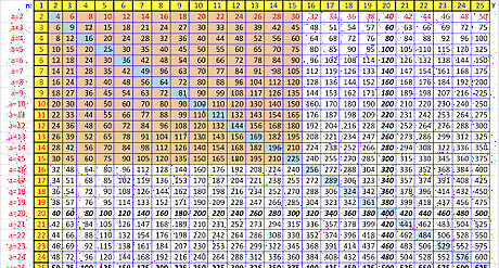
Here are the Multiplication Table and the Chart of a*n = x*y:


Comments
0 comment